RAxML hands-on session
Welcome to the RAxML hands-on session. I will assume that you are running some flavor of Linux/Unix operationg system and that you are familiar with some basic Linux/Unix commands. To get all test datasets, type "wget http://sco.h-its.org/exelixis/resource/download/hands-on/Hands-On.tar.bz2" or download here.Graphical user interface
You may also test the new graphical user interface of RAxML that is available hereStep 1: Download and installation
Go to Alexis github repository and download the latest RAxML version. When the download is completed type:unzip standard-RAxML-master.zip
This will create a directory called standard-RAxML-master Change into this directory by typing
cd standard-RAxML-master
Initially, we will need to compile the RAxML executables, if you don't know what a compiler is or why we need to do this, see here.
Because RAxML is available as sequential, vectorized, parallel, and vectorized parallel program (all included in the same source code) we will have to compile, that is, generate executables for various versions of RAxML.
To obtain the sequential version of RAxML type:
make -f Makefile.gcc
this will generate an executable called raxmlHPC. If you then want to compile an additional version of RAxML make always sure to type rm *.o before you use another Makefile, the *.o files. Assume, we are using a laptop with two cores and want to compile all RAxML versions that will run on it we would type:
- make -f Makefile.gcc -> generates a binary called raxmlHPC
- rm *.o
- make -f Makefile.SSE3.gcc -> generates a binary called raxmlHPC-SSE3, this is also a sequential version of RAxML that however exploits a type of very fine-grain parallelism in the processor. See here for more information on SSE3 and vector instructions.
- rm *.o
- make -f Makefile.PTHREADS.gcc -> generates a binary called raxmlHPC-PTHREADS that can run in parallel on several cores that share the same memory (that's the case on all common multi-core desktop and laptop computers). Pthreads are a library for generating and managing a specific sort of leight-weight processes which are called threads.
- rm *.o
- make -f Makefile.SSE3.PTHREADS.gcc -> generates a Pthreads version called raxmlHPC-PTHREADS-SSE3 of RAxML as described above, but it also uses vector instructions within each core/processor. Usually the vectorized versions of the code (with SSE3) are faster than the non-vectorized ones because more arithmetic instructions can be executed per processor clock cycle.
./raxmlHPC
or copy all the executables into our local directory of binary files, my username is stamatak so we would copy all executables into the respective binary directory by typing
cp raxmlHPC* ~stamatak/bin/
When this is done I can then execute RAxML in any diorectory by typing
raxmlHPC
without the ./ in fron of it. To get an overview of available commands type:
raxmlHPC -h
We will also need some tree visualization tool to look at the output trees. I always use Dendroscope because it can handle large trees and is easy to install. Please go to the dendroscope homepage and follow the installtion instructions provided there.
Step 2: Test Datasets
Here is a list of test datasets that we will use and need to download:- Alignment of binary characters
- Alignment of DNA characters
- a partition file that will allow us to partition the datasets into two partitions: one for the 1st and 2nd position and one for the 3rd DNA position
- another partition file that will allow us to partition the dataset into two partitions from position 1-30 and position 31-60
- a secondary structure file that will allow us to use RNA secondary structure models for this DNA dataset (essentially it would need to be RNA, but this is just an example so it doesn't matter)
- Alignment of protein characters
- Alignment of multi-state characters
- Alignment of DNA and protein characters
- a respective partition file
- A binary backbone constraint tree for our DNA dataset
- A multi-furcating constraint tree for our DNA dataset
Step 3: Getting Started
Let's get started with a simple ML search on binary data:raxmlHPC -m BINGAMMA -p 12345 -s binary.phy -n T1
and open the resulting tree called RAxML_result.T1 with Dendroscope. BINGAMMA tells RAxML that we are using binary data and we want to use the GAMMA model of rate heterogeneity. The file name appendix passed via -n is arbitrary, for this run all output files will be named RAxML_FileTypeName.T1 for instance. Every RAxML run will require a different run ID in order to avoid overwriting previous results.
We could also type:
raxmlHPC-SSE3 -m BINCAT -p 12345 -s binary.phy -n T2
CAT is a memory and time efficient approximation for the standard GAMMA model of rate heterogeneity. It is particularly convenient for saving memory on very large datasets. However, it should not be used for datasets with less than say 50-100 taxa. Also, it should not be confused with mixture models in phylogenetics. WARNING: Likelihood values obtained from the CAT model should not be used as a basis for comparing trees by means of their likelihood values!
As starting trees RAxML uses randomized stepwise addition parsimony trees, i.e., it will not generate the same starting tree every time. You can either force it by providing a fixed random number seed:
raxmlHPC -m BINGAMMA -p 12345 -s binary.phy -n T3
or by passing a starting tree
raxmlHPC -m BINGAMMA -t startingTree.txt -s binary.phy -n T4
If you want to conduct multiple searches for the best tree you can type:
raxmlHPC -m BINGAMMA -p 12345 -s binary.phy -# 20 -n T5
here RAxML will carry out 20 ML searches on 20 randomized stepwise addition parsimony trees.
We can now do the same thing for the DNA and protein data:
raxmlHPC -m GTRGAMMA -p 12345 -s dna.phy -# 20 -n T6
and
raxmlHPC -m PROTGAMMAWAG -p 12345 -s protein.phy -# 20 -n T7.
For protein data we may chose among a set of standard models with fixed transition rates that are typically estimated from a large number of real-world datasets: DAYHOFF, DCMUT, JTT, MTREV, WAG, RTREV, CPREV, VT, BLOSUM62, MTMAM, LG we may also chose to use empirical base frequencies drawn from the alignment (by essentially just counting the freuqency of occurence of the amino acids), rather than use the pre-defined base frequencies that come with the models:
raxmlHPC -m PROTGAMMAJTTF -p 12345 -s protein.phy -n T8
(DAYHOFFF, DCMUTF, JTTF, MTREVF, WAGF, RTREVF, CPREVF, VTF, BLOSUM62F, MTMAMF, LGF). Here we may also use the CAT approximation of rate heterogeneity again:
raxmlHPC -m PROTCATJTTF -p 12345 -s protein.phy -n T9.
A question that arises is of course which protein model to select. What I typically do is the following. I generate a reasonable reference tree and then just compute the likelihood scores (without conducting a tree search) under all available models. I then just use the model that yields the best score under GAMMA. There is also a perl script available to do this automatically here.
Note that, in more recent RAxML versions the best protein model with respect to the likelihood on a fixed, reasonable tree can also be
automatically determined directly by RAxML using the following commad:
raxmlHPC -p 12345 -m PROTGAMMAAUTO -s protein.phy -n AUTO
It is also possible to estimate a GTR model for protein data, but this
should not really be used on small datasets because there is not enough
data to estimate all 189 rates in the matrix:
raxmlHPC -p 12345 -m PROTGAMMAGTR -s protein.phy -n GTR
Here is the command to conduct a ML search on multi-state morphological datasets:
raxmlHPC -p 12345 -m MULTIGAMMA -s multiState.phy -n T10.
There
are different models available for multi-state characters that can be
specified via -K ORDERED|MK|GTR, the default is GTR so we just executed
a multi-state inference under the GTR model, for MK we can execute
raxmlHPC -p 12345 -m MULTIGAMMA -s multiState.phy -K MK -n T11
and for ordered states
raxmlHPC -p 12345 -m MULTIGAMMA -s multiState.phy -K ORDERED -n T12
Step 4: Bootstrapping
Now let's conduct a simple bootstrap analysis. Initially, let's try to find the best-scoring ML tree for a DNA alignment. We refer to this as the best-scoring tree because the ML search problem is computationally hard and we can thus generally not find the optimal tree under ML for a given alignment.Let's execute:
raxmlHPC -m GTRGAMMA -p 12345 -# 20 -s dna.phy -n T13
This command will generate 20 ML trees on distinct starting trees and also print the tree with the best likelihood to a file called RAxML_bestTree.T13. Now we will want to get support values for this tree, so let's conduct a bootstrap search:
raxmlHPC -m GTRGAMMA -p 12345 -b 12345 -# 100 -s dna.phy -n T14
We need to tell RAxML that we want to do bootstrapping by providing a bootstrap random number seed via -b 12345 and the number of bootstrap replicates we want to compute via -# 100. Note that, RAxML also allows for automatically determining a sufficient number of bootstrap replicates, in this case you would replace -# 100 by one of the bootstrap convergence criteria -# autoFC, -# autoMRE, -# autoMR, -# autoMRE_IGN.
Having computed the bootstrap replicate trees that will be printed to a file called RAxML_bootstrap.T14 we can now use them to draw bipartitions on the best ML tree as follows: raxmlHPC -m GTRCAT -p 12345 -f b -t RAxML_bestTree.T13 -z RAxML_bootstrap.T14 -n T15.
This call will produce to output files that can be visualized with Dendroscope: RAxML_bipartitions.T15 (support values assigned to nodes) and RAxML_bipartitionsBranchLabels.T15 (support values assigned to branches of the tree). Note that, for unrooted trees the correct representation is actually the one with support values assigned to branches and not nodes of the tree!
We can also use the Bootstrap replicates to build consensus trees, RAxML supports strict, majority rule, and extended majority rule consenus trees:
- strict consensus: raxmlHPC -m GTRCAT -J STRICT -z RAxML_bootstrap.T14 -n T16
- majority rule: raxmlHPC -m GTRCAT -J MR -z RAxML_bootstrap.T14 -n T17
- extended majority rule: raxmlHPC -m GTRCAT -J MRE -z RAxML_bootstrap.T14 -n T18
Step 5: Rapid Bootstrapping
Because bootstrapping is very compute intensive, RAxML also offers a rapid bootstrapping algorithm that is one order of magnitude faster than the standard algorithm discussed above. To invoke it type, e.g.,:raxmlHPC -m GTRGAMMA -p 12345 -x 12345 -# 100 -s dna.phy -n T19
so the only difference here is that you use -x instead of -b to provide a bootstrap random number seed. Otherwise you can also chose different models of substitution and also use the bootstrap convergence criteria with rapid bootstrapping as well.
The nice thing about rapid bootstrapping is that it allows you to do a complete analysis (ML search + Bootstrapping) in one single step by typing
raxmlHPC -f a -m GTRGAMMA -p 12345 -x 12345 -# 100 -s dna.phy -n T20
If called like this RAxML will do 100 rapid Bootstrap searches, 20 ML searches and return the best ML tree with support values to you via one single program call.
Step 6: Partitioned Analyses
A common task is to conduct partitioned analyses. We need to pass the information about partitions to RAxML via a simple plain text file that is passed via the -q parameter. For a simple partitioning of our DNA dataset we can type:raxmlHPC -m GTRGAMMA -p 12345 -q simpleDNApartition.txt -s dna.phy -n T21
The file simpleDNApartition partitions the alignment into two regions as follows:
DNA, p1=1-30
DNA, p2=31-60
p1 and p2 are just arbitrarly chosen names for the partition. We also need to tell RAxML what kind of data the partition contains (see below). If we partition the dataset like this the alpha shape parameter of the Gamma model of rate heterogeneity, the empirical base frequencies, and the evolutionary rates in the GTR matrix will be estimated independently for every partition. If we type:
raxmlHPC -M -m GTRGAMMA -p 12345 -q simpleDNApartition.txt -s dna.phy -n T22
RAxML will also estimate a separate set of branch lengths for every partition. If we want to do a more elaborate partitioning by, 1st, 2nd and third codon position we can execute:
raxmlHPC -m GTRGAMMA -p 12345 -q dna12_3.partition.txt -s dna.phy -n T23
The partition file now looks like this:
DNA, p1=1-60\3,2-60\3
DNA, p2=3-60\3
Here, we infer distinct model parameters jointly for all 1st and 2nd positions in the alignment and separately for the third position in the alignment. We can of course also use partitioned datasets that contain both, DNA and protein data, e.g.:
raxmlHPC -m GTRGAMMA -p 12345 -q dna_protein_partitions.txt -s dna_protein.phy -n T24
the partition file looks as follows:
DNA, p1 = 1-50
WAG, p2 = 51-110
Here we are telling RAxML that partition p1 is a DNA partition (for which GTR+GAMMA will be used) and that partition p2 is a protein partition for which WAG+GAMMA will be used. Note that, the parameter -m is now only used to extract the desired model of rate heterogeneity which will be used for all partitions, i.e., we could also type:
raxmlHPC -m PROTGAMMAWAG -p 12345 -q dna_protein_partitions.txt -s dna_protein.phy -n T25
which will be exactly equivalent. If we want to use a different protein substitution model for p2 we may edit a partition file that looks like this:
DNA, p1 = 1-50
JTTF, p2 = 51-110
Now JTT with empirical base frequencies will be used. The format is analogous for binary partitions, e.g., assuming that p1 is a binary partition we would write
BIN, p1 = 1-50
and for multi-state partitions, e.g.,
MULTI, p1 = 1-50
Don't forget to specify your substitution model for multi-state regions via -K (the chosen model will then be applied to all multi-state partitions).
Step 7: Secondary Structure Models
Specifying secondary structure models for an RNA alignment works slightly differntly because we read in a plain RNA alignment and then need to tell RAxML by an additional text file that is passed via -S which RNA alignment sites need to be grouped together. We do this in a standard bracket notation written into a plain text file, e.g., our DNA test alignment has 60 sites, thus our secondary structure file needs to contain a string of 60 characters like this one:..................((.......))............(.........)........
The '.' symbol indicates that this is just a normal RNA site while the brackets indicate stems. Evidently, the number of opening and closing brackets mus match. In addition, it is also possible to specify pseudo knots with additional symbols: <>[]{} for instance:
..................((.......)).......{....(....}....)........
In terms of models there are 6-state, 7-state and 16-state models for accommodating secondary structure that are specified via -A. Available models are: S6A, S6B, S6C, S6D, S6E, S7A, S7B, S7C, S7D, S7E, S7F, S16, S16A, S16B. The default is the GTR 16-state model (-A S16). In RAxML the same nomenclature as in PHASE is used, so please consult the phase manual for a nice and detailed description of these models.
For our small example datasets we would run a secondary structure analysis like this:
raxmlHPC -m GTRGAMMA -p 12345 -S secondaryStructure.txt -s dna.phy -n T26
A common question is whether secondary structure models can also be partitioned. This is presently not possible. However, you can partition the underlying RNA data, e.g., use two partitions for our DNA dataset as before. What RAxML will do internally though is to generate a third partition for secondary structure that does not take into account that distinct secondary structure site pairs may stem from different partitions of the alignment.
Step 8: Using the Pthreads Version
Using the Pthreads version is fairly straight-forward. The only really important thing you need to know is that you should never run it with more threads (light-weight processes) than you have cores (processors/CPUs) available on your system! This may lead to serious performance degradation. Assume that you have 4 cores but start 5 threads. In this case two threads will be continously competing to get compute time on one core and thereby also slow down the remaining threads that will be waiting for the two adverseary threads to finish their dispute.In order to run the Pthreads version you just need to use the correct executable (raxmlHPC-PTHREADS or raxmlHPC-PTHREADS-SSE3) and specify one additional parameter, the number of threads you want to use via -T, e.g.:
raxmlHPC-PTHREADS -T 2 -p 12345 -m PROTGAMMAWAG -s protein.phy -n T27
this will run nicely on my laptop that has two cores. If you want to see them running type top and then 1 which will show you the computational load on all cores of your computer. You will see that both cores are running at almost 100% to compute likelihoods on trees.
Step 9: Constraint Trees
When you are passing trees to RAxML it usually expects them to be bifurcating. The rationale for this is that a multifurcating tree actually represents a set of bifurcating trees and it is unclear how to properly resolve the multifurcations in general. Also, for computing the likelihood of a tree we need a bifurcating tree, therefore resolving multi-furcations, either at random or in some more clever way is a necessary prerequisite for computing likelihood scores.I personally have s strong dislike for constraint trees because the bias the analysis a prior using some biological knwoledge that may not necesssarily represent the signal coming from the data one is analyzing. The only purpose for which they may be useful is to assess various hypotheses of monophyly by imposing constraint trees and then conducting likelihood-based significance tests to compare the trees that were generated by the various constraints.
Overall RAxML offers to types of constraint trees binary backbone constraints and multifurcating constraint trees.
In a backbone constraint we pass a bifurcating tree to RAxML whose structure will not be changed at all and just add those taxa in the alignment that are not contained in the binary backbone constraint to the tree via an ML estimate (see below).
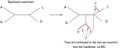
For our DNA dataset we may specify a backbone constraint like this: "(Mouse, Rat, (Human, Whale));" and type:
raxmlHPC-SSE3 -p12345 -r backboneConstraint.txt -m GTRGAMMA -s dna.phy -n T28
Multi-furcating constraints are slightly different in that they maintain the monophyletic structure of the backbone, but evidently taxa within a monopyhletic clade may be moved around. Also taxa that are not contained in the multi-furcating constrain tree which need not be comprehensive may be placed into any branch of the tree via ML.
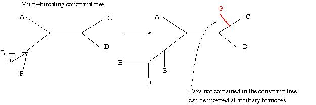
For our DNA dataset we can specify a multi-furcating constraint tree like this: "(Mouse, Rat, Frog, Loach, (Human, Whale,Carp));" and type:
raxmlHPC-SSE3 -p 12345 -g multiConstraint.txt -m GTRGAMMA -s dna.phy -n T29
Evidently, it doesn't make sense to specify a binary backbone constraint that contains all taxa (given that the backbone will remain fixed there is nothing to rearrange), while for multifurcating constraints it makes sense, for instance to resolve the multi-furcations.
A Frequent misconception about how constraint trees work in RAxML. One frequent problem users encounter is RAxML behavior when they use incomplete constraint trees, i.e., when the constraint does not contain all taxa in the alignment. Consider an alignment with 25 taxa in which you want to have enfore two phylogenetic groups for taxa A1, A2,...,A5 and B1, B2. Let's assume that the other taxa (not contained in the constraint) are called X1, X2, .... X17.
Now if you specify a constraint like this: "((A1,A2,A3,A4,A5),B1,B2);" it is not clear how the remaining taxa (X1,...,X17) shall behave. In RAxMl I have decided that they can be inserted anywhere in the tree and potentially within the monophyletic groups A and B. The property that is maintained (or shall be maintained if the implementation is correct) is that, in every tree using the above constraint, you will always find a branch that will split the taxon set such that taxa A1,...,A5 are on one side of that branch and taxa B1, B2 are on the other side of that branch. The positions of the taxa X1,...,X17 are completely irrelevant in this case, since your constraint only says something about A and B. If you don't want the X-taxa to appear within the groups A and B you will need to specify a comprehensive constraint (including all taxa) like this: "((A1,A2,A3,A4,A5),(B1,B2),(X1,X2,...,X17);".
Please have a look at the tree below that has been built with the constraint "((A1,A2,A3,A4,A5),B1,B2);" and convince yourself that it actually respects the constraint according to the definition used in RAxML:
Step 9.1 Constraining sister taxa
Now, if you want to constrain potential sister taxa to strict monophyly, e.g., mouse and rat, while other taxa will be allowed to freely move around the tree during ML topology optimization, you could do the following: Assume Mouse and Rat shall be forced to be monophyletic, you can specify a multi-furcating backbone constraint (containing, e.g., all taxa in dna.phy as follows: "(Cow, Carp, Chicken, Human, Loach, Seal, Whale, Frog, (Rat, Mouse));" and store this in a file monophylyConstraint.txt. Then you can call:raxmlHPC-SSE3 -p 12345 -g monophylyConstraint.txt -m GTRGAMMA -s dna.phy -n T29monophyly
Assume that now you would like to force the Frog and the Mouse to be monophyletic, here you'd write: "(Cow, Carp, Chicken, Human, Loach, Seal, Whale, Rat, (Frog, Mouse));" and store this in a file called, e.g., weirdMonophyly.txt and execute:
raxmlHPC-SSE3 -p 12345 -g weirdMonophyly.txt -m GTRGAMMA -s dna.phy -n T29weird_monophyly
If the constraint doesn't make much sense (e.g., Frog sister to Mouse) you will get a worse likelihood score for this and then use likelihood tests to determine wether the two alternative hypotheses yield trees with significantly differnt LnL scores.
Step 10: Outgroups
An outgroup is essentially just a tree drawing option that allows you to root the tree at the branch leading to that outgroup. If your outgroup contains more than one taxon it may occur that the outgroups cease to be monophyletic, in this case RAxML will print out a respective warning. For our DNA dataset we can specify a single outgroup like this:raxmlHPC-SSE3 -p 12345 -o Mouse -m GTRGAMMA -s dna.phy -n T30
If we want Mouse and Rat to be our ougroups we just type:
raxmlHPC-SSE3 -p 12345 -o Mouse,Rat -m GTRGAMMA -s dna.phy -n T31
Advanced Topics
- Using the hybrid MPI/Pthreads version of RAxML
- Computing RF and weighted RF topological distances between trees
- Evolutionary placement of short sequence reads
- Site weight calibration algorithms
- Accurate fossil placement
- Phylogenetic binning
- Computing the memory requirements of an alignment
- When to use the single-precision version of RAxML
- How does bootstopping work ?
- Checkpointing RAxML
- The -F and -D options